Facebook Prophet is based on an additive model where non-linear trends are fit with yearly, weekly, and daily seasonality,
plus holiday effects. It is designed to forecast time series data that have strong seasonal effects and several seasons of
historical data. It is robust against missing data and shifts in the trend and handles outliers very well.
It is open source software
released by Facebook’s Core Data Science team .
It is available for download on CRAN
and PyPI .
This blog explains a typical time series forecasting use case of predicting stock prices. First section shows how to acquire daily data of a blue-chip stock and
the necessary data wrangling. In the second section, we fit the FBProphet model on the processed data and plot some predictions.
The third and last section shows hyper-parameter tuning and cross-validation error.
Data Acquisition
There are various libraries to extract real time stock data. Yahoo finance, as being among the most famous, free with granularity of
1min, is used here. Below is the code to extract prices data from yahoo finance using REST calls.
    symbol='^GSPC',
    data_range='5m',
    data_interval='1d'
    session = requests.Session()
    retry = Retry(connect=10, backoff_factor=0.3)
    adapter = HTTPAdapter(max_retries=retry)
    session.mount('http://', adapter)
    session.mount('https://', adapter)
    try:
         conn_url = 'https://query1.finance.yahoo.com/v8/finance/chart/{symbol}?range={data_range}&interval={data_interval}'
                     .format(**locals())
         res = session.get(conn_url)
         if res.status_code != 200:
            return None
        data = res.json()
    except requests.ConnectionError as e:
        print("OOPS!! Connection Error.")
        pass

    if data['chart']['result'] is None:
        return None

    body = data['chart']['result'][0]

    if 'timestamp' not in body:
        return None

    dt = datetime.datetime
    dt = pd.Series(map(lambda x: arrow.get(x).to('Europe/Vienna').datetime.replace(tzinfo=None), body['timestamp']), name='Datetime')

    df = pd.DataFrame(body['indicators']['quote'][0], index=dt)

    df_adj = pd.DataFrame(body['indicators']['adjclose'][0], index=dt)
    df['Datetime'] = df.index
    df['Adj_Close'] = df_adj['adjclose']
    df['Symbol'] = symbol
    df = df.reset_index(drop=True)
    df = df.loc[:, ('Datetime', 'Open', 'High', 'Low', 'Close', 'Volume', 'Symbol', 'Adj_Close')]

    df.head()
The curl url takes three parameters namely, symbol also called as ticker (^GSPC=S&P 500), data_range
is the history to observe and data_interval is the granularity of the historic data where
data_interval is in [1m, 2m, 5m, 15m, 30m, 60m, 90m, 1h, 1d, 5d, 1wk, 1mo, 3mo]. The above query gives the following data:
| Datetime |
Open |
High |
Close |
Low |
Volume |
Symbol |
Adj. Close |
| 2010-01-04 15:30:00 |
1116.56 |
1133.86 |
1116.56 |
1132.98 |
3.99+09 |
^GSPC |
1132.98 |
| 2010-01-05 15:30:00 |
1132.66 |
1136.63 |
1129.66 |
1136.52 |
2.49+09 |
^GSPC |
1136.52 |
| 2010-01-06 15:30:00 |
1135.70 |
1139.18 |
1133.94 |
1137.14 |
4.97+09 |
^GSPC |
1137.14 |
To understand the structure of the data in more details, please consult candlestick charts.
The input to FBProphet is always a dataframe with two columns: ds and y. The ds (datestamp) column should be of a format
expected by Pandas, ideally YYYY-MM-DD for a date or YYYY-MM-DD HH:MM:SS for a timestamp.
The y column must be numeric, and represents the measurement we wish to forecast.
We would like to predict the closing price of S&P 500 at end of the each trading day. Let us therefore,
formulate the dataset accordingly.
    df_price = pd.DataFrame()
    df_price['ds'] = pd.to_datetime(df.Datetime)
    df_price['y'] = df['Close']
    df_price = df.reset_index(drop=True)
    df_price
| ds |
y |
| 2010-01-04 15:30:00 |
1116.560059 |
| 2010-01-05 15:30:00 |
1129.660034 |
| 2010-01-06 15:30:00 |
1133.949951 |
In this example, we try to predict the last 7 days of closing prices in our dataset, i.e., our prediction window is the last 7 days.
Let us therefore, arrange the data into train and test sets accordingly as follows:
    test_window = 7 ### days
    max_rows = df_price.shape[0]

    df_train = df_price[0:max_rows-test_window]
    df_test = df_price[max_rows-test_window:max_rows]
    df_train.shape, df_test.shape
Price Predictions
The next step is now to fit the model and validate predictions. For that the followings are the necessary libraries that are needed to
be installed and imported. Prophet follows the sklearn model API.
    import os, sys
    import pandas as pd
    import numpy as np

    from sklearn.metrics import mean_absolute_error, mean_squared_error
    from sklearn.metrics import accuracy_score, confusion_matrix, classification_report, roc_curve, auc

    import time
    from dateutil.relativedelta import *
    import matplotlib.pyplot as plt

    import warnings; warnings.simplefilter('ignore')
    pd.set_option('display.max_colwidth', 5000)
    pd.set_option('display.max_rows', 100)

    from fbprophet import Prophet
    from fbprophet.diagnostics import cross_validation
    from fbprophet.diagnostics import performance_metrics
    from fbprophet.plot import add_changepoints_to_plot
The initialization function takes a few parameters, the most relevant for this example
are daily_seasonality and changepoint_prior_scale. All real world time
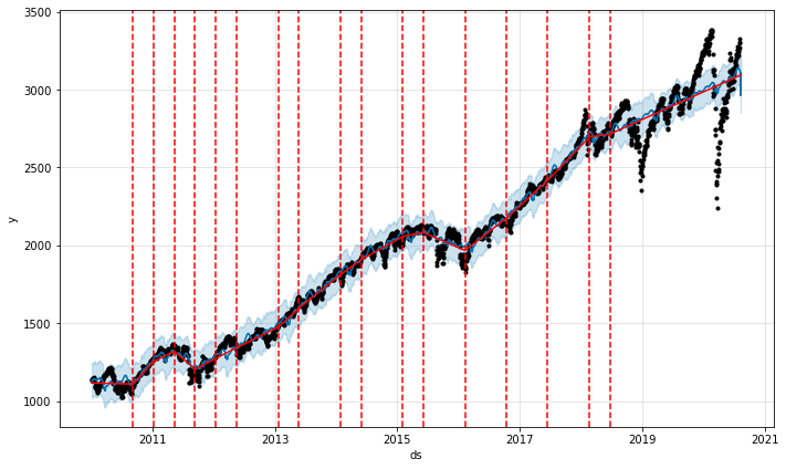
series data has abrupt frequency changes in their trajectories called as changepoints. By default, Prophet will automatically detect
these changepoints and will allow the trend to adapt appropriately. However, in case one wishes to have
finer control over this process (e.g., Prophet missed a rate change, or is overfitting rate changes in the history),
then the above two parameters can be used.
The algorithm detects changepoints by first specifying a large number of potential changepoints at which the rate is allowed to change.
It then puts a sparse prior on the magnitudes of the rate changes (equivalent to L1 regularization) - this essentially means that Prophet has a
large number of possible places where the rate can change, but will use as few of them as possible.
If the trend changes are being overfit (too much flexibility) or underfit (not enough flexibility), the
strength of the sparse prior can be adjusted using the input argument changepoint_prior_scale.
By default, this parameter is set to 0.05 and increasing it will make the trend more flexible.
The default changepoints are only inferred for the first 80% of the time series and can be
changed using the changepoint_range=0.9, which increases the range for the first 90% of the time series.
Changepoints are indicated by the vertical lines in the prediction plot of FBProphet's plot function.
From our experience, we have used the following initialization paramters:
    ml_prophet = Prophet(changepoint_prior_scale=0.15, daily_seasonality=True)
    ml_prophet.fit(df_train)
    fcast_time=test_window
    df_forecast = ml_prophet.make_future_dataframe(periods= fcast_time, freq='D', include_history=True)
    # Forecasting - call the method predict
    df_forecast = ml_prophet.predict(df_forecast)
    df_forecast[['ds', 'yhat', 'yhat_lower', 'yhat_upper']]
| ds |
y_hat |
yhat_lower |
yhat_upper |
| 2010-01-04 15:30:00 |
1128.733330 |
1022.160441 |
1244.312529 |
| 2010-01-05 15:30:00 |
1132.685715 |
1030.294347 |
1238.238948 |
| 2010-01-06 15:30:00 |
1132.784571 |
1133.889024 |
1025.191926 |
| ... |
... |
... |
... |
Here y_hat is the predicted y value and yhat_lower and yhat_upper
are the respective lower and upper bounds of the predictions. Subtracting y and y_hat then gives
the forecast errors.
The library also provides a comprehensive approach for the automatic cross validation over the range of historical cutoffs using its built-in
cross_validation function. This is done by selecting cutoff points in the history, and for each of them fitting the model using data
only up to that cutoff point. This requires more detailed explanation which can be read from the original documentation
here. In our example,
we specified the forecast horizon (horizon), and then optionally the size of the initial training period (initial)
and the spacing between cutoff dates (period).
By default, the initial training period is set to three times the horizon, and cutoffs are made every half a horizon.
    cutoffs = pd.to_datetime(['2020-07-23', '2020-08-01', '2018-08-15'])
    df_cv = cross_validation(ml_prophet, initial='2600', period='100 days', horizon = '14 days')
    df_cv.tail()
| ds |
y_hat |
yhat_lower |
yhat_upper |
y |
cutoff |
| 2020-07-30 15:30:00 |
3114.707554 |
3010.465909 |
3222.002343 |
3246.219971 |
2020-07-22 15:30:00 |
| 2010-07-31 15:30:00 |
3112.901688 |
3004.031733 |
3219.895283 |
3271.120117 |
2020-07-22 15:30:00 |
| 2020-08-03 15:30:00 |
3105.692670 |
3001.133212 |
3213.548760 |
3294.610107 |
2020-07-22 15:30:00 |
| 2020-08-04 15:30:00 |
3106.124081 |
2995.353238 |
3216.300242 |
3306.510010 |
2020-07-22 15:30:00 |
| 2020-08-05 15:30:00 |
3102.633426 |
2996.846280 |
3211.951709 |
3327.770020 |
2020-07-22 15:30:00 |
    df_p = performance_metrics(df_cv)
    df_p
| horizon |
mse |
rmse |
mae |
mape |
mdape |
coverage |
| 2 days 00:00:00 |
5680.853666 |
75.371438 |
46.773511 |
0.020461 |
0.015112 |
0.681174 |
| 2 days 23:00:00 |
5663.192682 |
75.254187 |
47.126214 |
0.020517 |
0.016454 |
0.686235 |
| 3 days 00:00:00 |
6640.232355 |
81.487621 |
50.124588 |
0.022620 |
0.013984 |
0.562753 |
| 3 days 23:00:00 |
6378.344252 |
79.864537 |
49.632274 |
0.022236 |
0.013984 |
0.582996 |
| ... |
... |
... |
... |
... |
... |
... |
| 13 days 23:00:00 |
29132.386064 |
170.682120 |
92.513042 |
0.053439 |
0.019412 |
0.424342 |
| 14 days 00:00:00 |
41006.122383 |
202.499685 |
106.722591 |
0.063297 |
0.021616 |
0.395833 |
    fig = ml_prophet.plot(df_forecast)
    a = add_changepoints_to_plot(fig.gca(), ml_prophet, df_forecast)
The results can be further improved by adding additional parameters to Prophet function such as
holidays=None, daily_seasonality=True, weekly_seasonality=True, yearly_seasonality=True. Curious
readers are welcome to explore such additional options.
Hyper-Parameter Tunning
FBProphet takes several hyper-parameters which makes it challenging to fnd the best match among them, i.e., there
are infinite many combinations when considering the all range of input values for each variable. It is therefore,
more efficient to perform an automated search for these parameters. For that FBProphet provides the following one possible
example:
    import itertools

    param_grid = {
        'changepoint_prior_scale': [0.001, 0.01, 0.1, 0.5],
        'seasonality_prior_scale': [0.01, 0.1, 1.0, 10.0],
        'seasonality_mode' : ['additive', 'multiplicative'],
        'changepoint_range': [0.85, 0.90, 0.95]
    }

    # Generate all combinations of parameters
    all_params = [dict(zip(param_grid.keys(), v)) for v in itertools.product(*param_grid.values())]
    rmses = []  # Store the RMSEs for each params here

    # Use cross validation to evaluate all parameters
    for params in all_params:
        m = Prophet(**params).fit(df_price)  # Fit model with given params
        df_cv = cross_validation(m,  initial='2600', period='100 days', horizon = '7 days')
        df_p = performance_metrics(df_cv, rolling_window=1)
        rmses.append(df_p['rmse'].values[0])

    # Find the best parameters
    tuning_results = pd.DataFrame(all_params)
    tuning_results['rmse'] = rmses
    #print(tuning_results)
    best_params = all_params[np.argmin(rmses)]
    print(best_params)
    {'changepoint_prior_scale': 0.5,
     'seasonality_prior_scale': 1.0,
     'seasonality_mode': 'multiplicative',
     'changepoint_range': 0.95}
    mdl_prophet = Prophet(changepoint_prior_scale=0.5,
                          seasonality_prior_scale=1.0,
                          seasonality_mode= 'multiplicative',
                          changepoint_range=0.95)
    mdl_prophet.fit(df_train)
    fcast_time=9
    df_forecast = mdl_prophet.make_future_dataframe(periods=fcast_time, freq='D', include_history=True)
    df_forecast = mdl_prophet.predict(df_forecast)


    from matplotlib import pyplot as plt
    fig = df_prophet.plot(df_forecast)
    fig.set_size_inches(20, 16)
    plt.xlabel('yhat', fontsize=24)
    plt.ylabel('date', fontsize=24)
    plt.rcParams['xtick.labelsize']=8
    plt.rcParams['ytick.labelsize']=8
    a = add_changepoints_to_plot(fig.gca(), mdl_prophet, df_forecast)
The above method resembles grid search approach towards hyper-parameter tuning which is
most time consuming among all the three possibilities namely, random, grid and bayesian search methods.
Please stay tune to read our next post on bayesian hyper-parameter tuning.
Your email address will not be published.